Foundations of Data Science: Common Probability Distributions and Their Explanations
Probability distributions are as fundamental to statistics as data structures are to computer science. If you want to be a competent data scientist, understanding them is foundational. Sometimes, simple analysis can be done directly with scikit-learn without fully understanding probability distributions, just as you can manage a Java program without knowing hash functions. But this might lead to failures and bugs.
There are hundreds of probability distributions, but the most common ones are about 15. What are they? This article will introduce them one by one.
Definition: What is a Probability Distribution?
Probabilistic events happen all the time: whether it will rain, the arrival time of a bus, rolling a die, and so on. The outcomes of these events are: it drizzled today, the bus arrived in 3 minutes, the die rolled a 3. Previously, we could only talk about the likelihood of results. Probability distributions describe what we believe the probability of each outcome is, and sometimes knowing this is more interesting than simply showing which outcome occurred. They come in many shapes but only one size: the sum of probabilities in a distribution is always 1.
For example, flipping a fair coin has two outcomes: it lands on heads or tails. (Assuming it cannot land on its edge or be snatched by a bird mid-air). We believe the probability of heads is 1/2, or 0.5. The same applies to tails. This is the probability distribution for the two outcomes of a coin flip, and if you can understand this sentence, you’ve grasped the Bernoulli distribution.
Despite their various names, the common types of probability distributions are limited. Let’s look at their relationship diagram for a better understanding of how they relate and evolve. Save the image for quick reference.
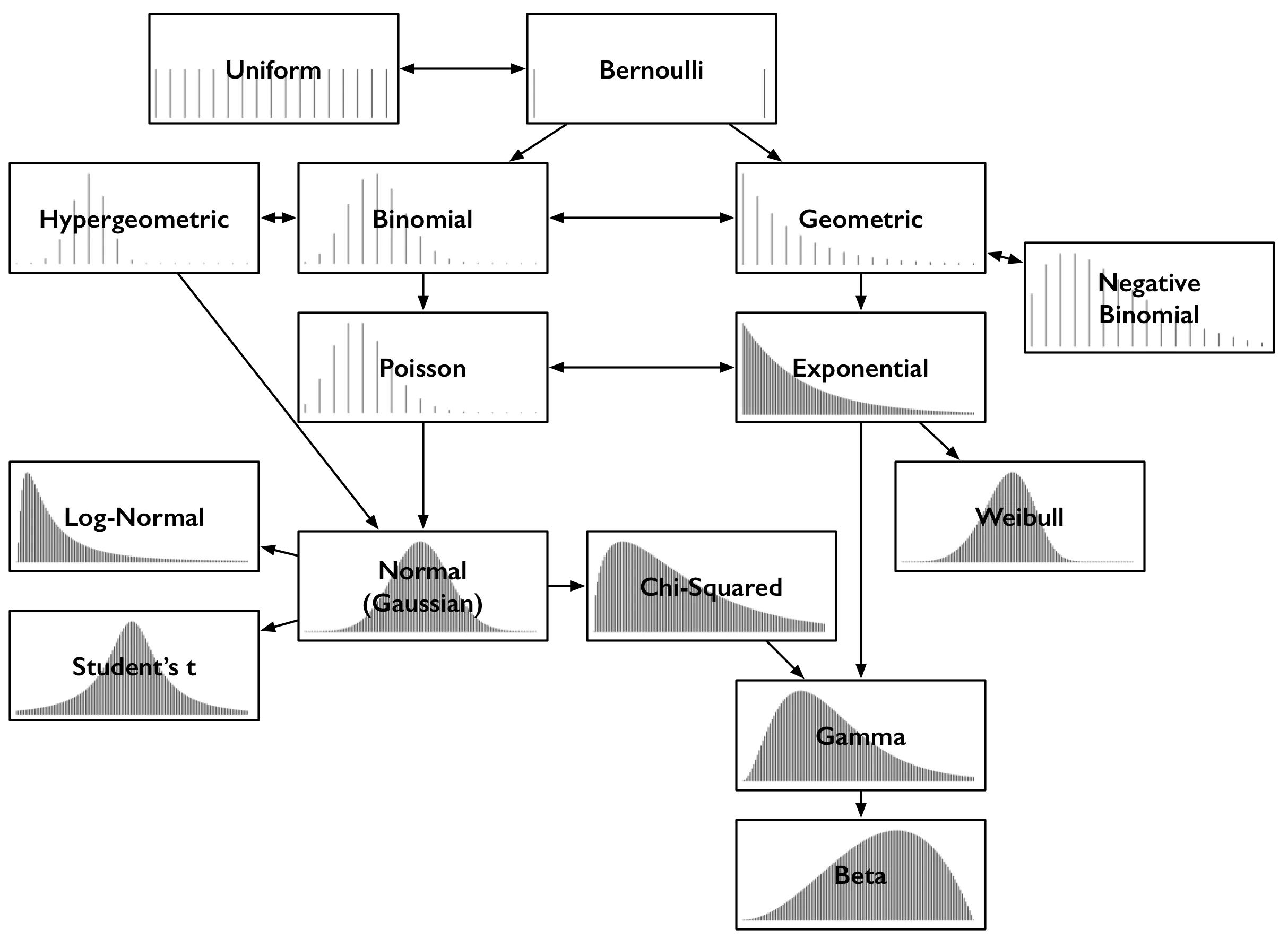
Each distribution is illustrated with an example of its Probability Density Function (PDF). So, the x-axis in each box is a set of possible numerical outcomes. The y-axis describes the likelihood or probability of the outcome. Since some distributions are discrete, their results must be integers like 0 or 1. These distributions are shown as sparse lines, where each result corresponds to a line, and the height of the line is the probability of that x-axis number appearing. Some are continuous, where results include all real numbers; these are shown as dense curves, and the area under various parts of the curve gives the probability. The sum of the heights of the lines and the area under the curve always total 1.
Bernoulli Distribution and Uniform Distribution
The Bernoulli distribution of a coin toss has only two discrete outcomes: heads or tails. From a distribution perspective, it can be viewed as a distribution over 0 and 1, representing the probability of heads and the probability of tails. In the example above, both outcomes have equal likelihood, which is what’s shown in the diagram. The Bernoulli PDF has two lines of equal height, representing the two equal outcomes 0 and 1 at both ends.
A Bernoulli distribution might represent less obvious outcomes, such as the result of flipping an unfair coin. In that case, the probability of heads is not 0.5, but some other value ‘p’, and the probability of tails is 1-p. Like many distributions, it is actually a family of distributions defined by parameters, such as ‘p’ here. When you think “Bernoulli,” just think “a (possibly unfair) coin flip.” This is the scenario for a probability distribution.
Next, imagine rolling a fair die. It has 6 faces, and each face has an equal probability. This is a Uniform distribution, characterized by its flat probability density. This is what a Uniform distribution is.
In summary, a Bernoulli distribution has only two possibilities: one event has a probability ‘p’, and the other has a probability ‘1-p’. The Uniform distribution is an extension of Bernoulli; it has multiple possibilities, but the probability of each possibility is the same. This is the Uniform distribution.
Binomial and Hypergeometric Distributions
The Binomial distribution can be thought of as the sum of results from multiple repetitions of a Bernoulli experiment. If you flip a fair coin 20 times, how many times do heads appear? This count follows a Binomial distribution. Its parameters are ’n’ (the number of trials) and ‘p’ (the probability of “success,” which is heads or 1 in this case). Each flip is the result or trial of a Bernoulli distribution. When counting the number of successes in coin flips or similar events, you arrive at the Binomial distribution, where each flip is an independent event and has the same probability of success.
Alternatively, imagine a black box with an equal number of white and black balls. Close your eyes, pick a ball, observe if it’s black, and then put it back. Repeat. How many times did you pick a black ball? This count also follows a Binomial distribution.
It makes sense to imagine this strange scenario because it simplifies the explanation of the Hypergeometric distribution. If, instead, the balls were not put back, then this would be a Hypergeometric distribution. It is admittedly similar to the Binomial distribution but not quite the same, because the probability of success (picking a black ball) changes as balls are removed. If the number of balls is very large relative to the number of draws, the distributions are similar because the chance of success changes little with each draw.
In summary, the Binomial distribution is the sum of results from repeated Bernoulli experiments with replacement, while the Hypergeometric distribution is the sum of results from repeated Bernoulli experiments without replacement.
Poisson Distribution
How many customers call a certain hotline per minute? If you consider each second as a Bernoulli trial, there are two outcomes: the customer doesn’t call (0), or the customer calls (1). This sounds like a binomial outcome. However, as everyone knows, two or even hundreds of people can call within the same second. So, we need to assume the probability of a call within 1 millisecond. In this case, the possibility of a call is much smaller, the probability is very low, but as long as there are two possibilities, with a success probability ‘p’, this is still a Bernoulli trial, just with a very small probability ‘p’. If time ’n’ approaches infinity (infinitely small time intervals), this limit is the Poisson distribution.
Like the Binomial distribution, the Poisson distribution is a distribution of counts – the number of times an event occurs. It is not parameterized by the probability of success ‘p’ and the number of trials ’n’, but by an average rate ‘λ’, which in this analogy is simply a constant np. When trying to count an event given a continuous rate of occurrence, you must think of the Poisson distribution.
Examples of Poisson distribution include: how many steamed buns are sold in a day, how many data packets arrive at a router, the number of customers arriving at a store, or the count of vehicles passing through a time period.
Geometric Distribution and Negative Binomial Distribution
Another distribution can be derived from the simplest Bernoulli trial. How many tails will appear before the first head when flipping a coin? The number of tails follows a Geometric distribution. Like the Bernoulli distribution, it is parameterized by ‘p’, the probability of success. Its parameter is not the number of failures; the result is the number of failures.
If the Binomial distribution asks “How many successes?”, the Geometric distribution asks “How many failures until success?”
The Negative Binomial distribution is a simple generalization of the Geometric distribution. It describes the number of failures until ‘r’ successes, not just 1 (which is the Geometric distribution). Therefore, it is also parameterized by ‘r’. Sometimes, it is described as the number of successes until ‘r’ failures. This conversion simply means the event definition is different, with one being the probability of heads and the other being the probability of tails; these are essentially the same.
Exponential Distribution and Weibull Distribution
Returning to the hotline calls: How long do you have to wait for the next customer? The distribution of waiting times sounds like it would be geometric, because every second without a call is like a failure, until the second a customer finally calls. The number of failures is like the number of seconds with no calls, which is approximately the waiting time until the next call, but not quite. This is because waiting times are always in whole seconds, not exact times.
As before, segment the Geometric distribution into infinitely small time slices, and it will eventually become effective. You will get the Exponential distribution, which accurately describes the distribution of time until a call. This is a continuous distribution, and it’s the first time we encounter a continuous outcome here, as the result time doesn’t have to be a whole second. Like the Poisson distribution, it is parameterized by a rate ‘λ’.
The Binomial-Geometric relationship is similar to the Poisson-Exponential relationship: the Poisson distribution asks “How many events occur?”, while the Exponential distribution asks “How long until an event occurs?”. Given that the count of an event follows a Poisson distribution, the time between events follows an Exponential distribution with the same rate parameter ‘λ’. The correspondence between these two distributions is crucial when discussing them.
When considering the “time until an event occurs,” perhaps “time until failure,” you should think of the Exponential distribution. In fact, this point is so important that there is a more general distribution to describe failure times, which is the Weibull distribution. The Exponential distribution is appropriate when the failure rate is constant, while the Weibull distribution can model failure rates that increase (or decrease) over time. The Exponential distribution is just a special case of the Weibull.
Normal, Lognormal, t-test, and Chi-Squared
The Normal distribution, also known as the Gaussian distribution, is perhaps the most important. Its bell-shaped structure is easily recognizable. Like the natural logarithm ’e’, it is a curious and special entity that emerges from seemingly simple origins. Take a bunch of values from any distribution (arbitrary distribution), and sum them up. The distribution of their sum follows (approximately) a Normal distribution. The more values you sum, the more closely their sum’s distribution matches the Normal distribution. (Note: The underlying distributions must be independent and well-behaved; only then will the sum tend towards a Normal distribution.) Regardless of the underlying distribution, it will converge to a Normal distribution.
This is known as the Central Limit Theorem, and you must know what this theorem is and what it means.
In this sense, it relates to all distributions. However, it specifically relates to the sum of events. The sum of Bernoulli trials follows a Binomial distribution, and as the number of trials increases, this Binomial distribution becomes more like a Normal distribution. The same applies to the Hypergeometric distribution. The Poisson distribution (an extreme form of the Binomial) also approaches the Normal distribution as its rate parameter increases.
If the logarithm of an arbitrary random variable follows a Normal distribution, then this is a Lognormal distribution. In other words, if you take the natural exponential of any Normally distributed value, you get a Lognormal distribution. Another way to put it is, if the sum of a certain distribution follows a Normal distribution, then that distribution is a Normal distribution.
The t-distribution is the basis of the t-test, which many non-statisticians learn in other scientific fields. It is used to infer the mean of a Normal distribution and also approaches the Normal distribution as its degrees of freedom (parameter) increase. A notable feature of the t-distribution is its tails, which are fatter than those of the Normal distribution. The t-distribution is used to estimate the mean of a normally distributed population with unknown variance based on a small sample. If the population variance is known (e.g., when the sample size is sufficiently large), the Normal distribution should be used to estimate the population mean.
The Chi-squared test is a hypothesis test where the distribution of a statistic approximately follows a chi-squared distribution under the null hypothesis. When no other limiting conditions or explanations are provided, the chi-squared test generally refers to Pearson’s chi-squared test.
Conclusion
This article summarized different types of univariate probability distributions in statistics and their application scenarios. You can refer to this when you’re unsure which model to use for analyzing your data.
- 原文作者:春江暮客
- 原文链接:https://www.bobobk.com/en/712.html
- 版权声明:本作品采用知识共享署名-非商业性使用-禁止演绎 4.0 国际许可协议进行许可,非商业转载请注明出处(作者,原文链接),商业转载请联系作者获得授权。