Calculating Confidence Intervals Using Bootstrapping
Concept
A confidence interval (CI) is the range within which the population parameter lies with a certain confidence level. It is estimated based on the original observed sample, usually defined as 95%, commonly called the 95% confidence interval.
Why Use Confidence Intervals
Generally, the obtained samples are drawn by sampling, and the population is unknown. Thus, data obtained from the sample cannot directly reflect the population. To express how well the sample represents the population, confidence intervals come into play.
Calculation of Confidence Interval
Assuming a dataset follows a normal distribution, the standard normal distribution’s confidence interval corresponds to the following z-scores:
Confidence Interval  z-score
0.90                1.645
0.95                1.96
0.99                2.58
The calculation formula for the confidence interval is:
That is, the mean plus the z-score times the standard deviation divided by the square root of n gives the upper bound of the confidence interval; subtracting it gives the lower bound.
Application
After explaining so much, the most important part is how to use this in scientific research or data analysis. Recently, I saw an article using the bootstrapping method to plot the 95% confidence interval of a distribution. Here, I demonstrate with this problem.
First, Generating the Data
import numpy as np
import pandas as pd
import matplotlib.pyplot as plt
import seaborn as sns
np.random.seed(1024)
data_nor = np.random.normal(loc=1, scale=2, size=1000)
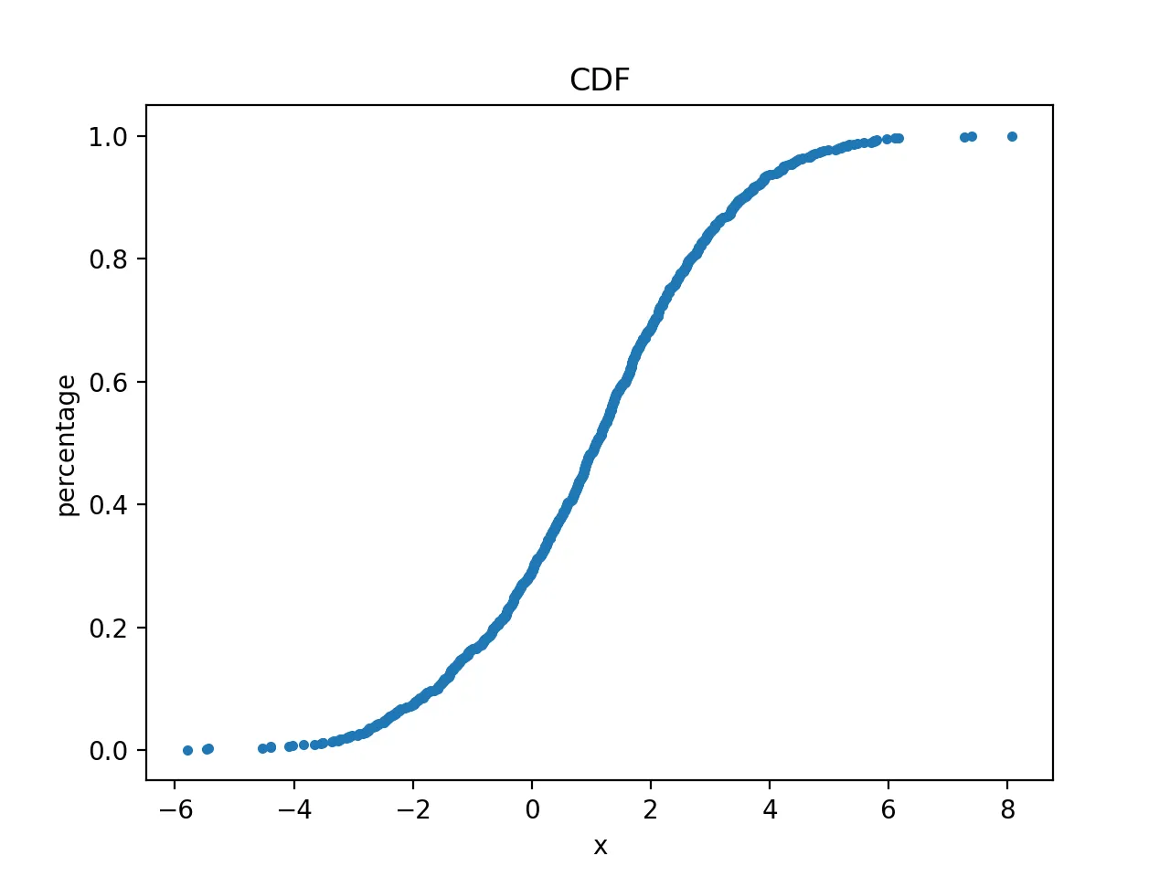
Viewing Its Cumulative Distribution Curve
Plotting the data against its proportion:
x = np.sort(data_nor)
n = len(x)
y = np.arange(1, n+1) / n
plt.plot(x, y, marker='.', linestyle="none")
plt.xlabel("x")
plt.ylabel("percentage")
plt.title("CDF")
plt.savefig("cdf.png", dpi=200)
plt.close()
The resulting plot is:
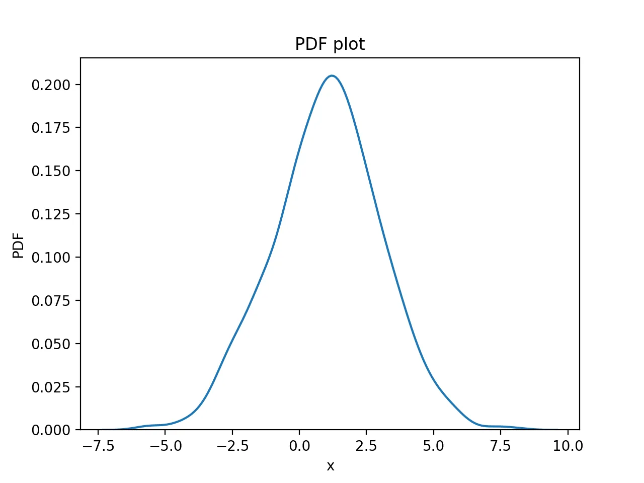
Viewing Its Density Curve
Smoothed curve of statistical values:
sns.distplot(data_nor, hist=False)
plt.xlabel("x")
plt.ylabel("PDF")
plt.title("PDF plot")
plt.savefig("pdf.png", dpi=200)
plt.close()
The plot is:
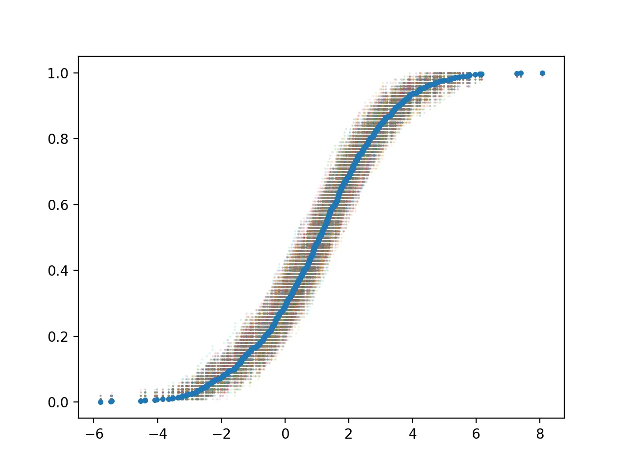
Generating Background Data Randomly via Bootstrapping and Calculating Confidence Interval
By randomly sampling 100 values from data_nor 10,000 times, the confidence interval is calculated. Random samples are plotted with transparency to highlight the original data and show the bootstrapped samples and confidence intervals.
# First plot the original data as the middle curve
plt.plot(x, y, marker='.', linestyle="none")
bs_mean = []
for i in range(10000):
    bs_sample = np.random.choice(data_nor, size=100)
    x = np.sort(bs_sample)
    bs_mean.append(np.mean(x))
    n = len(x)
    y = np.arange(1, n+1) / n
    plt.scatter(x, y, s=1, marker='.', alpha=0.2)
plt.savefig("bs.png", dpi=200)
plt.close()
The resulting plot is:
The distribution of the means after bootstrapping is plotted, with vertical lines marking the 2.5% and 97.5% confidence intervals. The confidence interval can be directly calculated using np.percentile.
plt.hist(bs_sample, bins=0.1, density=True)
plt.axvline(x=np.percentile(bs_sample, [2.5]), ymin=0, ymax=1, label='2.5%', c='y')
plt.axvline(x=np.percentile(bs_sample, [97.5]), ymin=0, ymax=1, label='97.5%', c='r')
plt.xlabel("x")
plt.ylabel("PDF")
plt.title("BS PDF")
plt.savefig("percent.png", dpi=200)
plt.close()
The plot is:
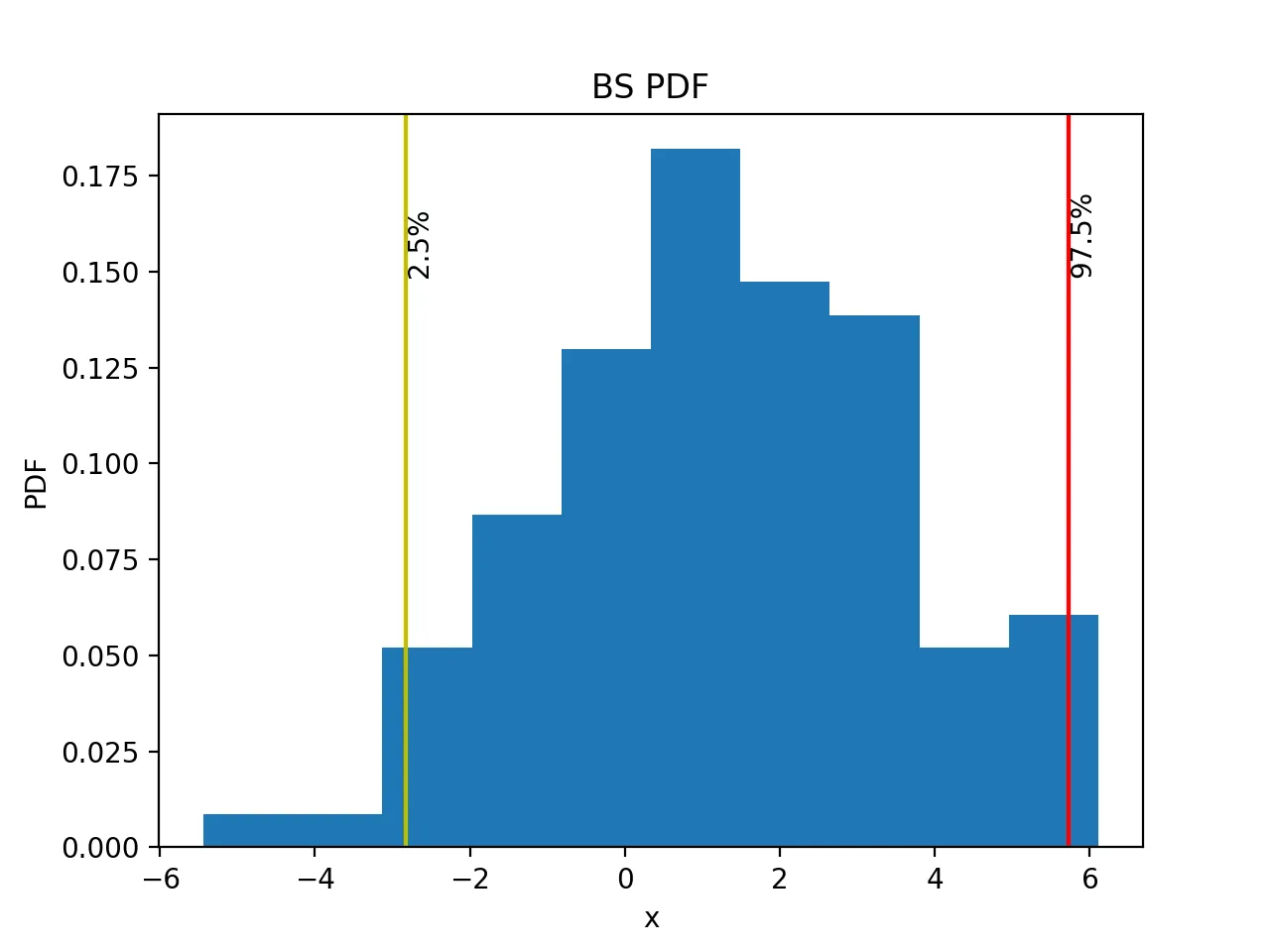
The 95% confidence interval is (-2.67366335, 4.18761485).
Summary
This article introduced confidence intervals and how to use bootstrapping to generate background data and calculate its confidence interval.
- 原文作者:春江暮客
- 原文链接:https://www.bobobk.com/en/838.html
- 版权声明:本作品采用知识共享署名-非商业性使用-禁止演绎 4.0 国际许可协议进行许可,非商业转载请注明出处(作者,原文链接),商业转载请联系作者获得授权。