K-Means Clustering and Implementation with sklearn

This article will explain the principles and applications of the K-Means clustering method from both mathematical and coding perspectives.

Cluster analysis allows us to find groups of similar samples or features, where the correlations between these objects are stronger. Common uses include grouping samples based on different gene expression patterns or grouping genes based on classifications of different samples.
This article will introduce the k-means clustering algorithm:

• Basic concepts of k-means clustering
• Mathematical principles behind the k-means algorithm
• Advantages and disadvantages of k-means
• Implementation using the scikit-learn package
• Visualization of clustering
• Selecting the optimal k

Basic Concepts of k-means Clustering

k-means is an efficient unsupervised clustering method originally used in signal processing. It aims to partition n observations into k clusters, where each observation belongs to the cluster with the nearest mean (cluster center or centroid), forming a group.
It is easy to confuse k-means with another clustering method from supervised learning called k-nearest neighbors (KNN), so care should be taken.

Mathematical Principles Behind the k-means Algorithm

Given a set of observations (left(x_1, x_2, ldots, x_nright)), where each observation is a d-dimensional real vector, k-means clustering aims to partition the n observations into k (≤ n) sets (S = {S_1, S_2, ldots, S_k}) to minimize the within-cluster sum of squares (WCSS) (i.e., variance) and maximize between-cluster differences. Formally:

where (u_i) is the mean of (S_i).
This formula is equivalent to minimizing the pairwise squared differences within the same cluster:

Advantages and Disadvantages of k-means

Advantages:

1. Simple principle and fast implementation
2. Good clustering performance
3. High interpretability of the algorithm
4. Only requires tuning the number of clusters k

Disadvantages:

1. Difficult to select the value of k
2. Hard to converge on non-convex datasets
3. Uses iterative methods that only guarantee local optima
4. Sensitive to noise and outliers

Implementation Using scikit-learn

First, randomly generate classified data, then perform clustering using the KMeans function:

import matplotlib.pyplot as plt
import pandas as pd
import seaborn as sns
from sklearn.datasets import make_blobs
from sklearn.cluster import KMeans

# from 春江暮客

x,y = make_blobs(n_samples=150, n_features=2,centers=3, cluster_std=0.5,shuffle=True, random_state=1024)
km = KMeans( n_clusters=3, init='random',n_init=10, max_iter=300, tol=1e-04, random_state=1024)
y_km = km.fit_predict(x)

Visualization of Clustering

The KMeans clustering results can be visualized using matplotlib or seaborn.

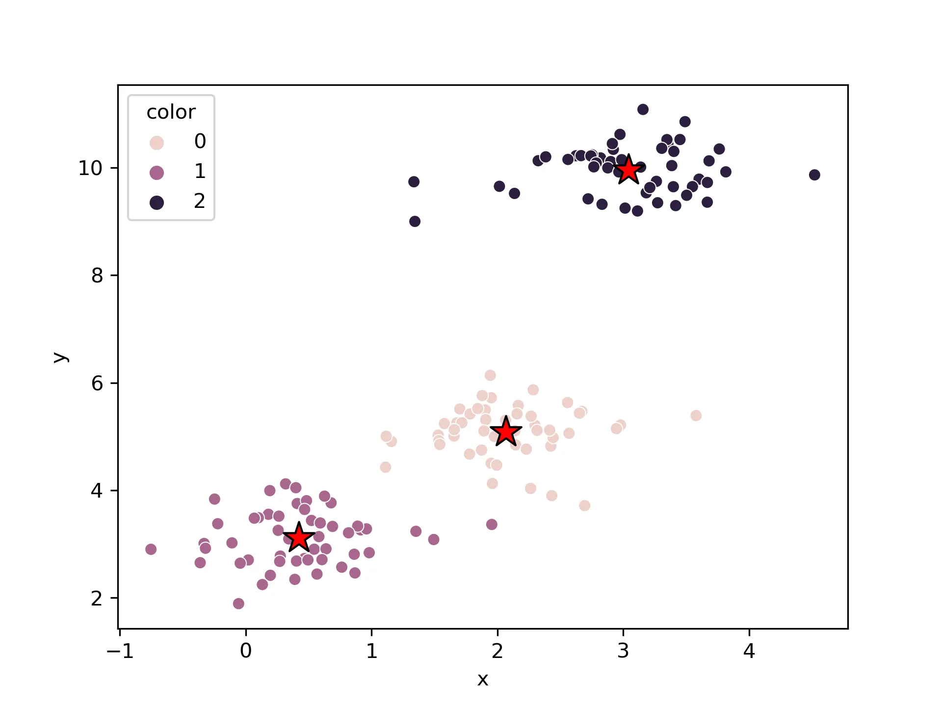
First, using seaborn:

# seaborn

df = pd.DataFrame(x,columns=["x","y"])
df["color"] = y_km
sns.scatterplot(data=df,x="x",y="y",hue="color", markers="color")
# Plot cluster centers
plt.scatter(
    km.cluster_centers_[:, 0], km.cluster_centers_[:, 1],
    s=250, marker='*',
    c='red', edgecolor='black',
    label='center'
)

Result:

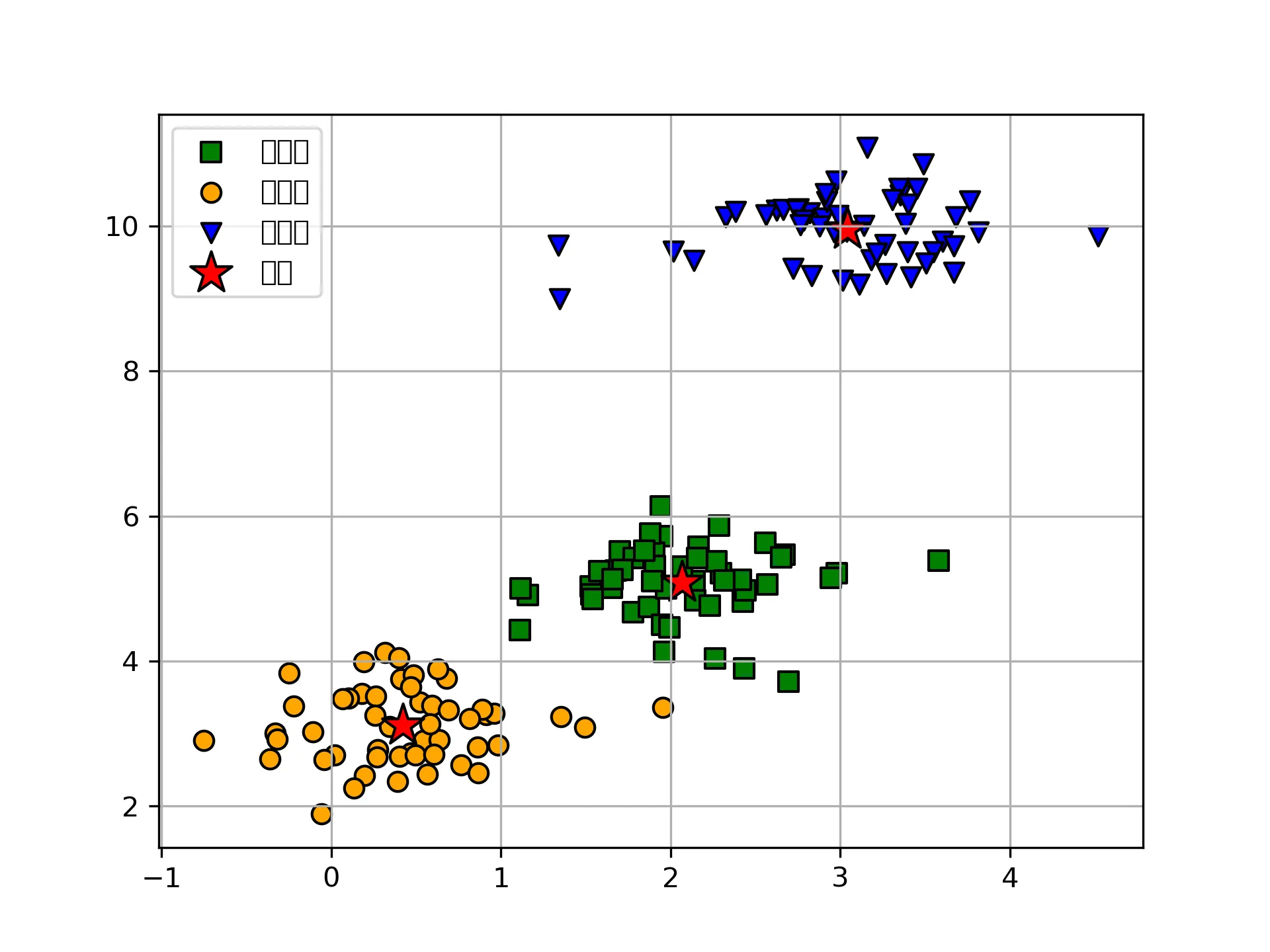
Next, directly using matplotlib:

# matplotlib
plt.scatter(
    x[y_km == 0, 0], x[y_km == 0, 1],
    s=50, c='green',
    marker='s', edgecolor='black',
    label='cluster1'
)

plt.scatter(
    x[y_km == 1, 0], x[y_km == 1, 1],
    s=50, c='orange',
    marker='o', edgecolor='black',
    label='cluster2'
)

plt.scatter(
    x[y_km == 2, 0], x[y_km == 2, 1],
    s=50, c='blue',
    marker='v', edgecolor='black',
    label='cluster3'
)

# Plot cluster centers
plt.scatter(
    km.cluster_centers_[:, 0], km.cluster_centers_[:, 1],
    s=250, marker='*',
    c='red', edgecolor='black',
    label='center'
)
plt.legend(scatterpoints=1)
plt.grid()
plt.show()

Result:

Selecting the Optimal k

For our generated data, the k-means clustering effect is very good. However, as mentioned earlier,
k-means is highly influenced by the choice of k. In multidimensional data, the number of clusters is not easy to judge. Theoretically, as k increases, within-cluster variance decreases, and between-cluster differences increase. Therefore, evaluating the best k in k-means clustering is very important. Here, the elbow method is used for evaluation.

distortions = []
for i in range(1, 11):
    km = KMeans(
        n_clusters=i, init='random',
        n_init=10, max_iter=300,
        tol=1e-04, random_state=1024
    )
    km.fit(x)
    distortions.append(km.inertia_)

# Plot
plt.plot(range(1, 11), distortions, marker='o')
plt.xlabel('Number of clusters')
plt.ylabel('Distortion')
plt.show()

Result:

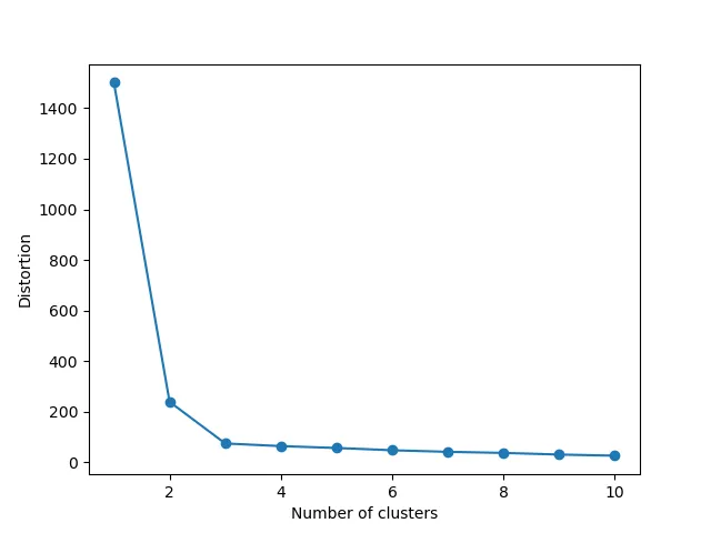
You can see that after k reaches 3, as k increases, y does not change drastically, so k=3 is the ideal number of clusters for this data.

Summary

This article started from the principles, step-by-step performed classification using sklearn, visualized the clustering effect using matplotlib and seaborn, and finally provided a method to find the optimal number of clusters.